Solving the 2D Cartesian Helmholtz Equation with Octave (Example 1)

Consider the following equation:

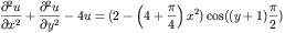
Defined on a Cartesian grid say [0,2]x[-1,3]. With boundary conditions given by

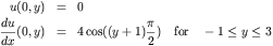
and

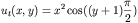
This is an inhomogenous Helmholtz equation with an exact solution given by

To solve this with "hwscrtg" is really quite simple. The limits of the Cartisian domain ([0,2]x[-1,3]) are supplied in the variables A,B,C, and D. The number of cells to decompose each domain (for the finite difference grid) are denoted M for x-dimension and N for the y-dimension. One is required to compute vectors representing each (non-periodic) boundary condtion and assign them to arrys that are passed in to the code. The arrays are denoted BDA, BDB, BDC, and BDD depending on the boundary at which the boundary conditions are specified (e.g. BDA corresponds to Dirchlet or Neumann boundary conditions on u(x=A,y)). It may be simpler to show an example driver function. 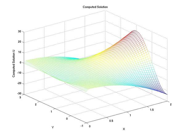Finally we can view the results of our hard work. First we plot the numerical solution obtained with the octave code

Next, we plot the difference between our numerically computed solution and the known exact solution given above

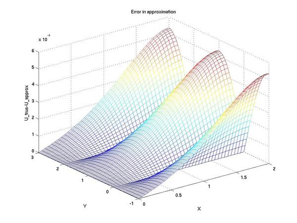
Since the magnitude is of order 1e-4, from this plot we can conclude that our implementation is working. To further test that the code is converging at the right rate we next plot the L^{\infty} error as a function of the grid spacing. The code to produce this plot is found here

John Weatherwax

Last modified: Fri Jul 14 04:07:38 EDT 2006