PDETWO Example 4:
Supposed one wanted to solve the following partial differential
equation representing fluid flow, diffusion and advection of a
tracer over a horizontal plane (y=0 with x arbitrary).
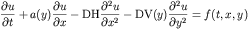
The above represents the time dependent concentration of a tracer
advecting with a velocity that depends on the height above the y=0
plane, a constant horizontal diffusion coefficient, and a variable
(y dependent) vertical diffusion coefficient. In addition we
will consider situations where the tracer source f has compact
support in space and possibly a time dependent strength in other
words the function f has a functional form given by
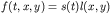
Here the function s(t) is the source strength and l(x,y) is the
compactly supported source location. We can consider the source
strength to be delta function if we want an impulsive introduction
of tracer.
We desire the solution of the PDE on the upper half plane with
homogeneous Neumann boundary conditions at y=0 and satisfying
radiation conditions on the other lateral boundaries. The
boundary condition on y=0 is then given by

While the other boundary conditions will be satisfied numerically
by taking a large enough numerical grid (say x in [-W,+W] and y in
[0,H]) and imposing Dirichlet boundary conditions given by

With initial conditions given by

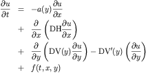
To write this equation in the form required for PDETWO i.e.
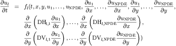
We can write it in the following way
This is quite simple to solve with the PDETWO gateway in octave.
First the user must specify an octave function "F.m" which
evaluates the right hand side of the PDE expressed in the PDETWO
standard form (given above). The input arguments to the octave
function F.m are t,x,y,u,ux,uy, duxx, and duyy. Here t is the
scalar time, x & y the scalar grid points, u is the unknown, ux is
the x derivatives of the unknown, uy is the y derivative of this
unknown, and duxx/duyy express the following derivatives

and

respectively. With the background we can write our F.m function
for evaluating the right hand side of our PDEs. In addition to
F.m, PDETWO requires the information on the horizontal and
vertical diffusion coefficients DXX and DYY. This is provided in
the form of two octave functions DIFF_H.m
and DIFF_V.m .
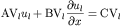
PDETWO requires two sets of boundary conditions one for each
domain boundary. The first must be specified on the East West
edges of the domain and has representative form given by
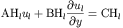
the second must be specified on the North South edges of the
domain and has representative form given by
To implement boundary conditions for PDETWO in octave we must
specify two boundary conditions functions. The vertical boundary
condition function will return AV, BV, and CV. The horizontal
boundary condition function will return AH, BH, and CH. Each are
allowed input arguments of t,x,y, and u (with the same meanings as
above). Here the horizontal boundary condition function is BNDRY_H.m, and the vertical boundary
condition function is BNDRY_V.m.
Finally the user must specify the initial conditions. In this
example the initial conditions are computed and passed into
pdecol.m. The initial conditions are compute with UINIT.m.
An initial condition function is not explicitly called by the
FORTRAN pdetwo code and is simply used for convenience.
Once this code is written a person can call "pdetwo.m". Here we
present an example pdetwo_Script.m driver file (don't be
intimidated by the comments).
For some specific functions, we can consider a situation where we
have a shear like advection term an isotropic diffusion (see the
functions above for the exact functional form)
Finally, we can reap the benefits of our work by viewing the
solution to our problem (shown here as profiles of the intensity
of our tracer taken at a series of times):
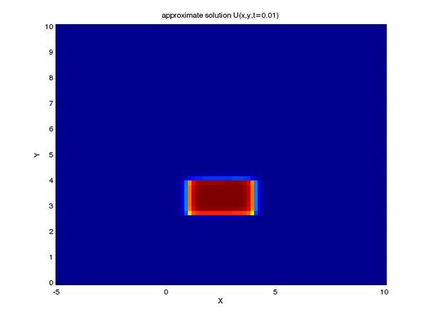
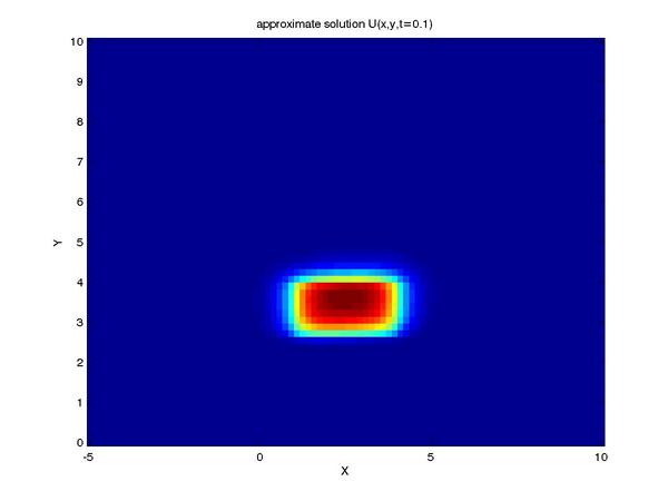
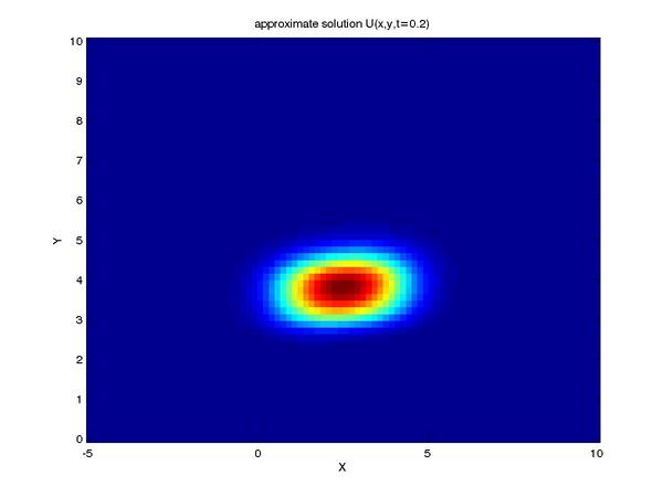
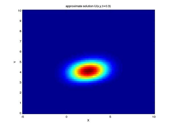
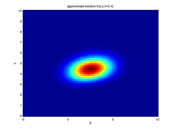
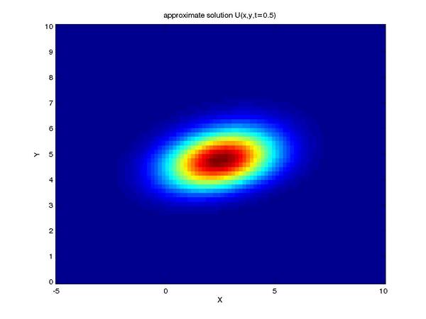
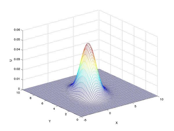
One can see the advection term begin to shear the tracer profile
as time progresses.
John Weatherwax
Last modified: Wed Jul 12 21:09:37 EDT 2006