TD learning using the grid world example. Here we compare several variants of the problem.
Some words on how I implemented these problems. The images below are shown in matrix format so that the index "i"
runs downward. The starting location is the state (4,1) while the ending location is the state (4,6).
The wind that affects the adjent is the value of the wind
before the adjent takes a step, thus when stepping from no wind into a region of wind there is no
additional displacement due to the wind. Also stepping off the grid world is allowed if the subsequent "wind" or
stocastic step takes the adgent back to a valid grid cell. If the agent steps off, the grid the code adjust each component
as needed and puts the adgent back to a valid location. The consequence of these facts is that the learning algorithm
often uses the fact that it can step off this grid and get carried back to a valid location via the wind in finding
optimal policies. This is talked about in more detail below. In each of the examples below I ran 10 millian episodes
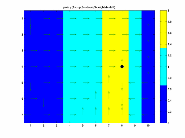
The first is the original example presented in the book and solved when running the code windy_gw.m.
The next plot is the sample polcy obtained when running the driver script. From each given grid location the
arrows point in the direction the greedy policy with respect to the learned action value function Q would point.
Starting from the start location in matrix notation at (4,1) and following the location of the arrows (and taking the
wind affect into account) we see that the policy selected is the same one as
presented in the book.

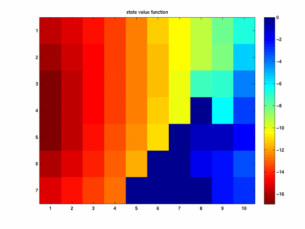
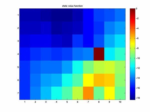
We next present the greedy state value function for this example. Numerically the value estimated for the
state value function is the "cost-to-go" the cost that the algorithm must pay to get to the finish when starting
at the given grid cell. From the given image the cost-to-go is about 17, or it take the agent about 17 steps to get
to the ending location on this task.

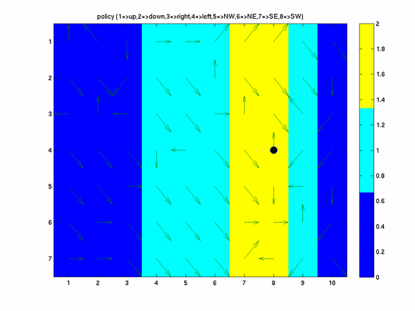
When the agent can take diagonal (or kings) moves the greedy policy derived looks like the following

In this case we can see that the adgent takes the path initially heading south east and then uses the fact that
he can step off of the grid and let the wind carry him back to the grid.
Here it should be noted that since we have to run our codes with a finite number of episodes some state in the grid
world are not sampled very many times. The consequence of this fact is that while we are plotting the greedy policy
for each grid cell if the agent did not actually visit that cell many times during all of its episodes then the policy
estimate in that cell may be quite poor. Two immedate fixes for this could be to run more episodes (assuming our
episodes sample the entire state space) or to initialy start our algorithm in state we are curious about exploring.
This is the method of exploring starts. For toy problems like this we could certainly start our agent at any
given location we desired and correspondingly inprove the policy estimate for that state. The estimated state value function
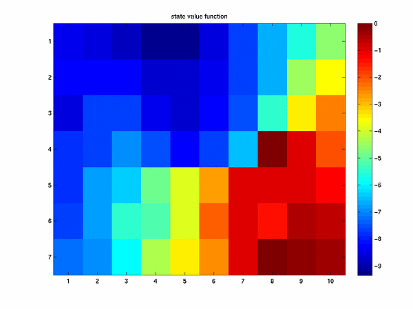
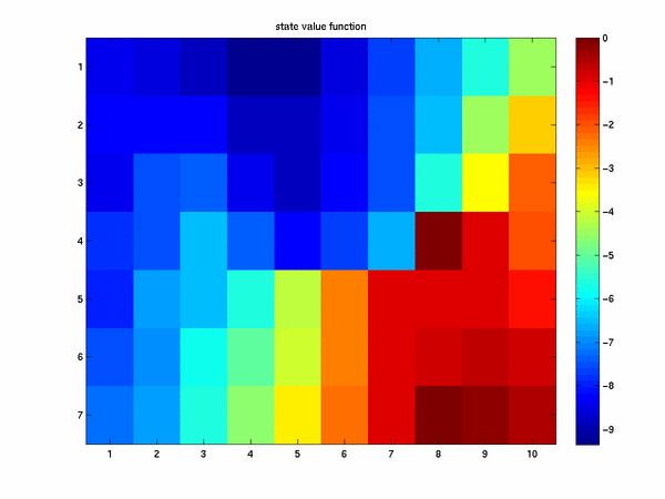
with 8 actions looks like

Where we see with the addition of kings moves we have a reduced cost-to-go and can reach our goal in fewer steps. Now we can reach
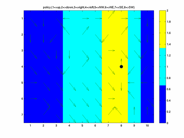
our goal in about 8.35 steps. If we are allowed a wind action state the greedy policy looks like the following

Here we see that the policy choosen is to use the wind when the agent gets to the location (6,6). The wind at
that location (two units upward) carries us directly into our target state. The corresponding state value function given by

We would expect that with more options avable namely that of chooseing a wind action we should be able to get to our goal
in a fewer number of steps. Thus we expect that the cost-to-go metric should be smaller. This is indeed true for the starting state.
The number of steps in each episode when we add a wind state is about 8.33 which is slightly smaller than the previous
case.
Finally, if we have a stochastic wind applied we expect to have to take more steps to get to our goal and
our policy looks like

and our state value function approximation looks like

We can see that it is harder to get to our goal in this case and that in fact it takes on average more
attemps. The code run_all_gw_Script.m when run will also compute the average number of timesteps
for each of the four methods. For 10,000 episodes this gives 17 steps for the original grid world, 9 steps
for the modification with kings moves, 9 steps for the modification with kings moves and a wind action, and
16.3 steps for the stochastic grid world problem.
John Weatherwax
Last modified: Sun May 15 08:46:34 EDT 2005
