Solving Partial Differential Equations with Octave
PDECOL
This is the first release of some code I have written for solving
one-dimensional partial differential equations with Octave. The types of
equations that can be solved with this method are of the following form
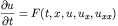
Here u can be a vector of unknowns depending on both space and
time. The spatial domain x is finite i.e. [a,b]. Here u_x is the
first partial derivative of the vector of unknowns and u_xx is the
vector of second partial derivatives, u_t is the vector of time
derivatives. Boundary conditions depend on the partial
differential equation (PDE) solved and are imposed in the octave
code as equations of the following form

Here b and z are user defined vector valued functions. The
initial conditions are specified for each component of u at the
initial time t_0. These initial conditions must be consistent
with the boundary conditions above. The user must specify octave
functions (with a very similar format to Matlab functions)
defining each of the functions described above for the specific
problem at hand. As such it is very easy to modify and solve
various different PDES. One can use the same functional call and
just change the octave functions references. Various examples of
this use are provided in the software below. The code is
currently a C++/octave API wrapper that calls the core solution
routine PDECOL described in the paper:
Algorithm 540: PDECOL, General Collocation Software for Partial Differential Equations
by N. K. Madsen, R. F. Sincovec
ACM Transactions on Mathematical Software (TOMS), Volume 5 Issue 3 (September 1979)
The algorithm is based on the method of lines and uses a finite
element collocation procedure with B-splines as its basis
elements. The polynomial order of the splines is an input
parameter. The allowable values are from (2 to 20). The ordinary
differential equations that result from a B-spline basis and the
imposed collocation can be integrated with either of two main
methods: Adams' methods (of order between 1 and 12) and backwards
differentiation methods (of order between 1 and 5).
Examples:
- The first example from the Madsen and Sincovec paper (using
octave) is given here. This is a rather complicated nonlinear
system of partial differential equations. In addition, included
in the source code below, are all of the additional examples from
this paper.
- If anyone finds this software helpful please send me an example
of its use, I would be happy to put it here.
Misc:
The license in the ACM code only allows non-commercial usage of
their codes. This license is too restrictive for the Free Software
Foundation GNU copyleft and therefore the code cannot be included
in the mainstream Octave sources. This license does however
permit usage of this software for educational purposes.
Please reference this software in any publications that
result from its use. A sample bibtex entry is below
    @misc{weatherwaxPDECOLG,

      author = "J L. Weatherwax",

      title  = "Software for solving PDE's with Octave",

      text   = "PDECOLG: An Octave Gateway Routine to pdecol.f",

      year   = "2005",

      url    = "http://web.mit.edu/wax/www/Software/pdecol.html"

    }
I should mention that I am very interested in having people use
this software and as such would be very willing to help get people
started using it. As always, please send any comments to the
address below.
-
The version
1.2 has all working examples from the Madsen and Sincovec paper.
-
The version
1.1 has a few minor bugs fixed over version 1.0. Specifically, the C++ code was
modified to return the initial condition along with the solution at the requested time.
Previous version didn't return the initial condition.
-
The version
1.0 code is effectively finished. It has had several
enhancements to improve readability and functionality of the
sections of the code users will interact with and more extensive
verification using of many of the examples from the paper above.
These examples are included in this release.
-
The version 0.9
code now allows the specified PDE to be define as octave functions.
In addition, the directory EG1 has a simple example of its use.
-
The version 0.1
code does work but is rather primitive in many
ways. The main restriction is that it still requires the user
code his/her partial differential equations, initial conditions,
and boundary conditions as described above in FORTRAN. This
version does allow easy parameter variations such as the number of
grid points, and does all memory allocation once the problem
definition FORTRAN is coded. The requirement of FORTRAN is a
major drawback. I've decided to release this anyways and begin
development on a version that will not require any FORTRAN coding.
This should be coming shortly.
Installation
General Notes:
The code was compiled on a 686 athalon chip
and thus should not need to be recompiled if you are using a
similar chipset. If this is not the case to rebuild the function
you will need a FORTRAN 77 compiler and a C++ compiler in addition
to the mkoctfile script to produce the dynamically linked function
pdecolg.oct.
More information about dynamically linked functions for octave can
be found in the: "Dal Segno al Coda" found here.
MacOS X:
Special thanks to Marcus Vinicius for
providing these excellent instructions.
Linux/Unix:
To run all the examples provided you first must extract the source
into a local directory. In this example, lets assume that you
downloaded a file named "PDECOL.x.y". Where x and y are the major
and minor version numbers PDECOL distribution. First unzip and
untar the distribution using
      gunzip PDECOL.x.y.tar.gz

      tar -xvf filename.tar
Where filename is the name of the version of code downloaded.
Next, change into the newly created directory
cd PDECOL.x.y
In that directory, one should see subdirectories containing the
various octave files used to specify the different PDE's. The
first numerical PDE example from the paper above is in the
subdirectory is named "EG1". To run the code corresponding to
this PDE definition. We must first insure that octave can find
these files and not any others with the same name. As such there
should be a file called .octaverc in this top most
directory. Open this file in an editor and change the line to
read (if it is not already)
LOADPATH = ['EG1//', LOADPATH];
Now start octave in this top most directory, with an invocation like
octave &
The LOADPATH command will set the path so that when
octave is started in the given directory it will find the required
pdecol_Script.m in the EG1 directory and no other.
Then at the octave prompt type
pdecol_Script
and the given PDE will be solved numerically for you with a few
plots produced.
Windows:
I developed the PDECOL package on a Linux system
and have never tested it on Windows, but it should work with if
the proper compilers are provided and you remake the dynamically
liked function pdecolg.oct. See the discussion above. If you are
able to get this to work I would be happy to hear about it
including tricks you had to know or perform to get everything to
work.
To Do:
- Finish Madsen/Sincovec examples EG3 and EG5.
- Make the passage of arguments to all of the user defined
functions easy.
- Include more examples of solved PDE's using this code on the
web (such as the examples above).
- Make it possible to pass in initial conditions as a matrix
in addition to the normal way through a user defined function.
- More complete and better documentation.
- If you are interested in working on any of these tasks please
contact me ... I'd love your help!!!
John Weatherwax
Last modified: Mon Sep 25 19:40:44 EDT 2006