PDEONE Example B: Shallow Water Flow
Supposed one wanted to solve the following system of partial
differential equations on the interval [-400,+400] (units are in
cm).
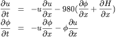
where u and  denote the horizontal velocity and depth of the fluid, H=H(x)
describes the surface over which the flow occurs, and g=980 is the
vertical acceleration due to gravity. These equations we
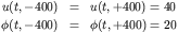
recognized as the shallow water equations. We desire the solution
of the PDE above with boundary conditions given by
denote the horizontal velocity and depth of the fluid, H=H(x)
describes the surface over which the flow occurs, and g=980 is the
vertical acceleration due to gravity. These equations we
recognized as the shallow water equations. We desire the solution
of the PDE above with boundary conditions given by
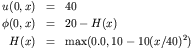
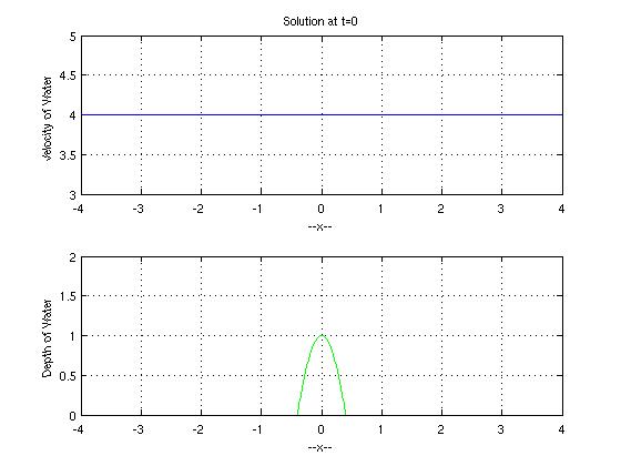
 With initial conditions and bottom topography given by
This corresponds to the second example in the original reference
to PDEONE (given above). This is quite simple to solve with the
pdeone gateway in octave. First the user must specify an octave
function "F.m" which evaluates the right hand side of the PDE
expressed in the following form
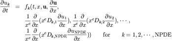
The incoming arguments to the octave function F.m are t,x,u,ux,
and duxx. Here t is the scalar time, x the scalar grid point, u a
vector of the NPDE unknowns, ux a vector of the x derivatives of
these unknowns, and duxx is a matrix expressing the
following derivatives
With the background we can write our F.m function for evaluating the right hand
side of our PDEs. In addition to F.m, PDEONE requires the
information on the diffusion coefficients D. This is provided in
the form of a function
D.m.
The routine "F.m" calls another octave function d_bottom_H.m to implement the derivative of
the bottom topography.
PDEONE requires the boundary conditions of the form

To implement this in octave we must specify three boundary
functions with input arguments t,x, and u (with the same meanings as
above):
BNDRY_ALPHA.m,
BNDRY_BETA.m, and
BNDRY_GAMMA.m.
Finally the user must specify the initial conditions. In this
example these are specified with the function shallow_init.m, where the bottom is described
in the octave function bottom_H.m. The two inputs to the initial
condition function are t and x. Here t is a scalar input of time
but in this case x is a vector of grid points where the initial
conditions are desired. Note, that to work properly this function
must be vectorized meaning that it can return a matrix
(of dimension [NPDE,Number of Grid Points]) of initial
conditions.
Once this code is written a person can call "pdeone.m". Here we
present an example pdeone_Script.m driver file. Note: Since
this problem is in Cartesian the constant c=0. Since this is the
default, there is no need to specify anything additional.
Finally, we can reap the benefits of our work by viewing the
solution to our problem:
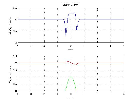
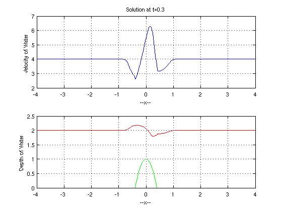
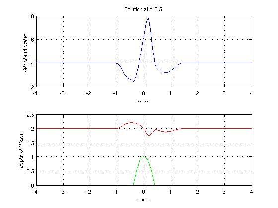
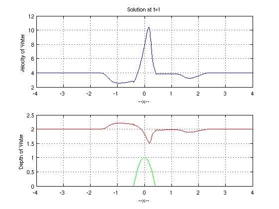
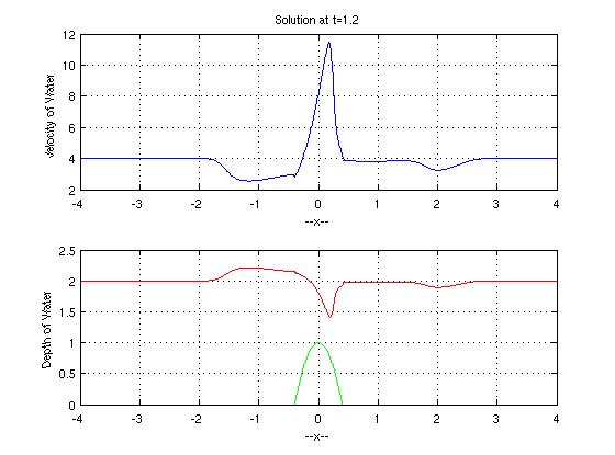
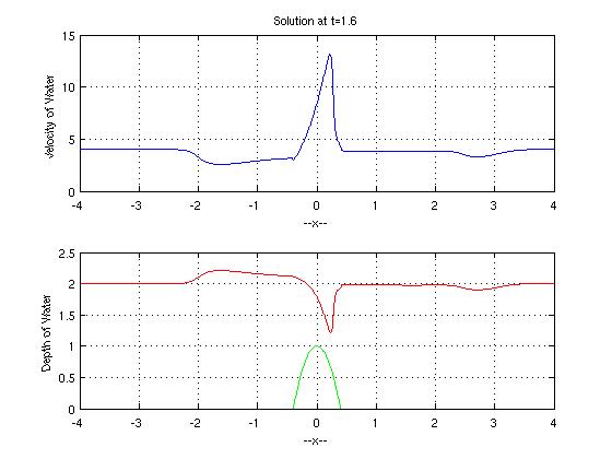
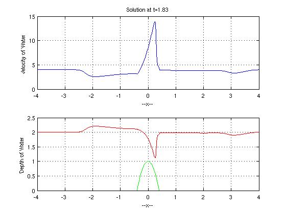 Note the downstream shock that develops. This last plot is a
replica of the plot given in the Sincovec and Madsen paper and is
itself a duplicate of Figure 14b found in
Nonlinear shallow fluid flow over an isolated ridge
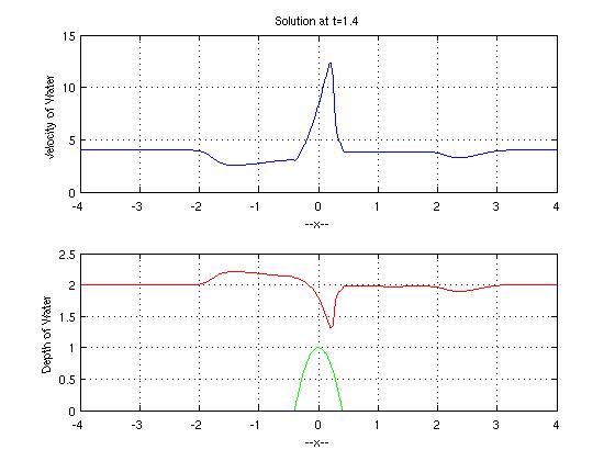
Note the downstream shock that develops. This last plot is a
replica of the plot given in the Sincovec and Madsen paper and is
itself a duplicate of Figure 14b found in
Nonlinear shallow fluid flow over an isolated ridge
by D. D. Houghton and A. Kashara
Comm. Pure Appl. Math. Vol. 21 (1968) 1-23
Due to the ease of use of the octave interface one can quickly
recognize the stationary shock locations, refine the grid around
these locations and view the results.
John Weatherwax
Last modified: Sat Jan 7 10:58:30 EST 2006