Solving Partial Differential Equations with Octave
PDEONE + the Runge Kutta Chebyshev ODE integrator rkc.f
This is the first release of some code I have written for solving
one-dimensional partial differential equations with Octave. The types of
equations that can be solved with this method are of the following form
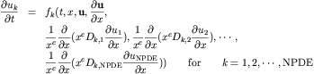
Here the vector u is a vector of unknowns that depends on both
space and time. The spatial domain x is finite i.e. [a,b]. Here
u_x is the first partial derivative of the vector of unknowns and
the second derivative information is specified by specifying the
"diffusion" functions D. The diffusion coefficients "D" can be
functions of x,t, and u. In addition, the constant c above can be
0, 1, or 2 depending on whether the problem is specified in
Cartesian, cylindrical, or spherical coordinates. Boundary
conditions depend on the partial differential equation (PDE)
solved and are imposed in the octave code as equations of the
following form

Here  ,
,  , and
, and  are user defined vector
valued functions which may depend on t and u if
are user defined vector
valued functions which may depend on t and u if  but only functions of
x otherwise. The initial conditions are specified for each
component of u at the initial time t_0. These initial conditions
don't necessarily have to be consistent with the boundary
conditions above.
but only functions of
x otherwise. The initial conditions are specified for each
component of u at the initial time t_0. These initial conditions
don't necessarily have to be consistent with the boundary
conditions above.
To solve PDE's with PDEONE in octave the user must specify octave
functions (with a very similar format to Matlab functions)
defining each of the functions described above for the specific
problem at hand. As such it is very easy to modify and solve
various different PDES. One can use the same functional call and
just change the octave functions references. Various examples of
this use are provided in the software below. The code is
currently a C++/octave API wrapper that calls the core solution
routine PDEONE described in the paper:
Algorithm 494: PDEONE, Solutions of Systems of Partial Differential Equations
by R. F. Sincovec and N. K. Madsen
ACM Transactions on Mathematical Software (TOMS), Volume 1 Issue 3 (September 1975)
As a check for errors I have be able to duplicate all of the
non-stiff results from that paper using the code provided here
(see below). Next one will find a subset of some of the examples
provided there. Note: all examples from that paper are
provided in this software delivery and work as well as the
included ODE solver can be expected to (see below).
Examples:
Note: that the reaction-diffusion example (above) is not from the
Sincovec and Madsen paper but was provided with the rkc ODE solver
as an example of is application in the method of lines.
I should mention that this version of PDEONE uses the numerical
ODE integrator "rkc.f" provided by Sommeijer, Shampine, and Verwer
which can be found on netlib. The ODE
solver used in the original Sincovec and Madsen paper was
Hindmarsh's integrator GEARB (see references in the paper above).
At the time of this programs development I couldn't find an
electronic version of this code and so used a Runge Kutta
Chebyshev ODE solver instead. Some comments about this solver are
in order. The rkc solver is an explicit method with very low
memory requirements and a quadratically growing stability region.
As such it is able to dynamically select, at each step, the most
efficient stable formula. These properties make it ideal for the
solution of parabolic partial differential equations
using the method of lines. In fact it is presented explicitly in
such a light in the paper below. The drawback in using such a
solver is that when the partial differential equation to be solved
is stiff (more hyperbolic than parabolic) this solver can fail.
When attempting to duplicate the results of the Sincovec and
Madsen paper on several of the examples this happened.
Practically, this means that the rkc solver takes unbearable a
long time while it iterates looking for an acceptable stability
region. This could be monitored by considering the output of the
variable MAXM but is currently not implemented yet. It should be
mentioned that as a quick fix often one can refine the grid or
extend the domain and the solver will be able to proceed. A more
permanent solution is to implement a stiff ODE solver (such as the
GEARB ODE solver). In the results presented here the rkc solver
performed as well as could be expected (which was quite well).
The Sommeijer, Shampine, and Verwer ODE solver "rkc" is described
in more detail in the following reference:
B.P. Sommeijer, L.F. Shampine and J.G. Verwer
RKC: an Explicit Solver for Parabolic PDEs.
Technical Report MAS-R9715, CWI, Amsterdam, 1997
The license in the ACM code only allows non-commercial usage of
their codes. This license is too restrictive for the Free Software
Foundation GNU copyleft and therefore the code cannot be included
in the mainstream Octave sources. This license does however
permit usage of this software for educational purposes.
Please reference this software in any publications that
result from its use. A sample bibtex entry is below
    @misc{weatherwaxPDEONEG,

      author = "J L. Weatherwax",

      title  = "Software for solving PDE's with Octave",

      text   = "PDEONEG: An Octave Gateway Routine to pdeone.f",

      year   = "2005",

      url    = "http://web.mit.edu/wax/www/Software/pdeone.html"

    }
I should mention that I am very interested in having people use
this software and as such would be very willing to help get people
started using it. As always, please send any comments to the
address below.
Code Versions:
-
The version 1.1 now allows the user to enter the
initial conditions as a matrix in addition to being able to
specify them as an octave function. This allows the user to use
this code to perform fractional splitting like techniques on their
equations. By this I mean one could decompose the initial problem
into two subproblems and solve the total problem by solving a
sequence of the two subproblems. In this sequence of subproblems
the solution to the firs problem is used as the initial condition
to the next problem in sequence and one must be able to specify
initial conditions as a matrix. There is a nice discussion of
this technique in Chapter 17 in Randall LeVeque's book "Finite
Volume Methods For Hyperbolic Problems".
-
The version 1.0 has all the examples from the
Sincovec and Madsen paper working and implemented, plus some
additional error checking.
-
The version 0.5 code has had a few bugs fixed
from the 0.2 release and many more examples from the Sincovec and
Madsen paper implemented.
-
The version 0.2
code works nicely and is able to duplicate the results from the
first example given in the paper references above. See the example.
Installation
General Notes:
The code was compiled on a 686 athalon chip
and thus should not need to be recompiled if you are using a
similar chipset. If this is not the case to rebuild the function
you will need a FORTRAN 77 compiler and a C++ compiler in addition
to the mkoctfile script to produce the dynamically linked function
pdeoneg.oct.
More information about dynamically linked functions for octave can
be found in the: "Dal Segno al Coda" found here.
Linux/Unix:
To run all the examples provided you first must extract the source
into a local directory. In this example, lets assume that you
downloaded a file named "PDEONE.x.y". Where x and y are the major
and minor version numbers PDEONE distribution. First unzip and
untar the distribution using
      gunzip PDEONE.x.y.tar.gz

      tar -xvf filename.tar
Where filename is the name of the version of code downloaded.
Next, change into the newly created directory
cd PDEONE.x.y
In that directory, one should see subdirectories containing the
various octave files used to specify the different PDE's. The
first numerical PDE example from the paper above is in the
subdirectory is named "EG1". To run the code corresponding to
this PDE definition. We must first insure that octave can find
these files and not any others with the same name. As such there
should be a file called .octaverc in this top most
directory. Open this file in an editor and change the line to
read (if it is not already)
LOADPATH = ['EG1//', LOADPATH];
Now start octave in this top most directory, with an invocation like
octave &
The LOADPATH command will set the path so that when
octave is started in the given directory it will find the required
pdeone_Script.m in the EG1 directory and no other.
Then at the octave prompt type
pdeone_Script
and the given PDE will be solved numerically for you with a few
plots produced.
Windows:
I developed the PDEONE package on a Linux system
and have never tested it on Windows, but it should work with if
the proper compilers are provided and you remake the dynamically
liked function pdeoneg.oct. See the discussion above. If you are
able to get this to work I would be happy to hear about it
including tricks you had to know or perform to get everything to
work.
To Do:
- Replace the ODE solver RKC with Hindmarsh's GEARB integrator
which (I now know) can be found with the PDETWO source code or another
implicit ODE solver.
- Make the passage of arguments to all of the user defined
functions easy.
- Include more examples of solved PDE's using this code on the web.
- More complete and better documentation.
- If you are interested in working on any of these tasks please
contact me ... I'd love your help!!!
John Weatherwax
Last modified: Sun May 14 13:14:06 EDT 2006